


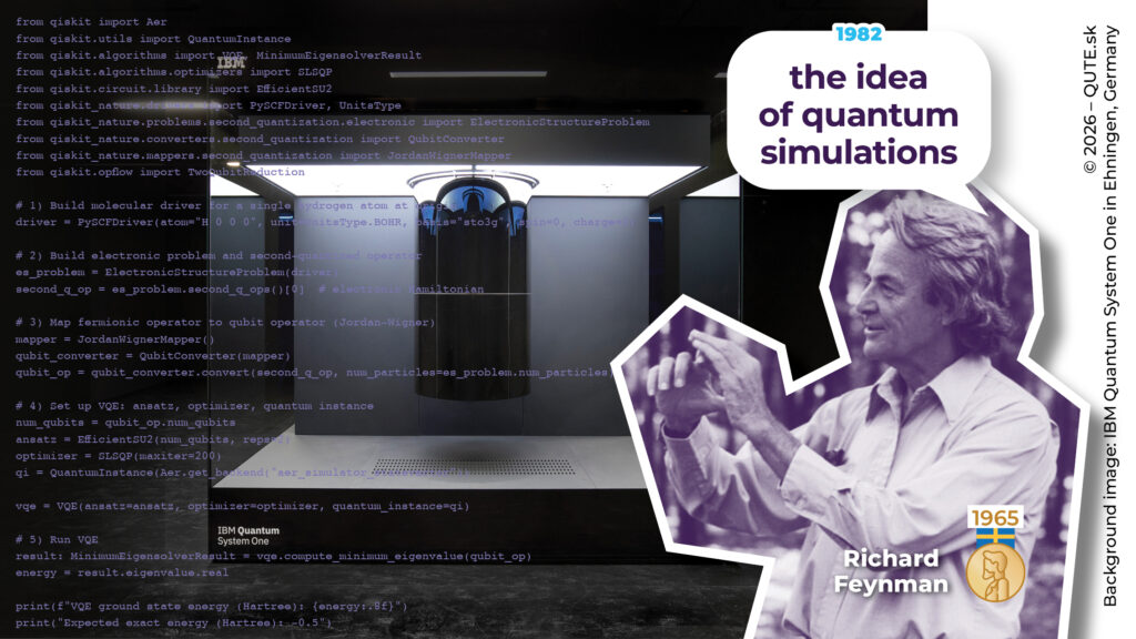
A quantum computing device in the NISQ era together with its simulation software. A list of such systems can be found on the English Wikipedia page “List of quantum processors.” The closest one is located at the Czech national supercomputing center IT4Innovations in Ostrava.
Computing quantum (in)equations
At school, we perceive physics as a subject dominated by formulas. But what do those describing the quantum world look like?
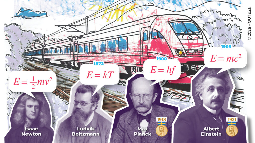
Do we calculate energy using the formula E = mv²/2, or E = mc²? With the exception of free particles, energy and velocity are quantum mechanically uncertain with respect to each other, meaning their values are not in any well-defined relationship. The quantum “formula” for energy, E = hf, where h = 6.62607015 × 10⁻³⁴ J·s is the Planck constant, introduces a new context for particles – frequency f. This is related to the fact that quantum systems are described as waves, whose dynamical characteristic is their frequency.
The equation for an object’s energy depends on the context of the physical theory that describes its behavior.
Laws of energy
Energy is one of the key concepts in physics. Yet it is not easy to say what energy actually is. One thing, however, is clear – total energy is conserved. This “mantra” is so important to physicists that whenever the conservation of energy seemed to be violated, new forms of energy – and even new physics – were introduced. This is how thermal energy entered our understanding of the world, as well as the prediction of the existence of neutrinos.
Even though total energy is conserved, energy is a quantity associated with changes in systems over time. Equations describe how energy transforms from one form to another and how the values of other physical parameters change.
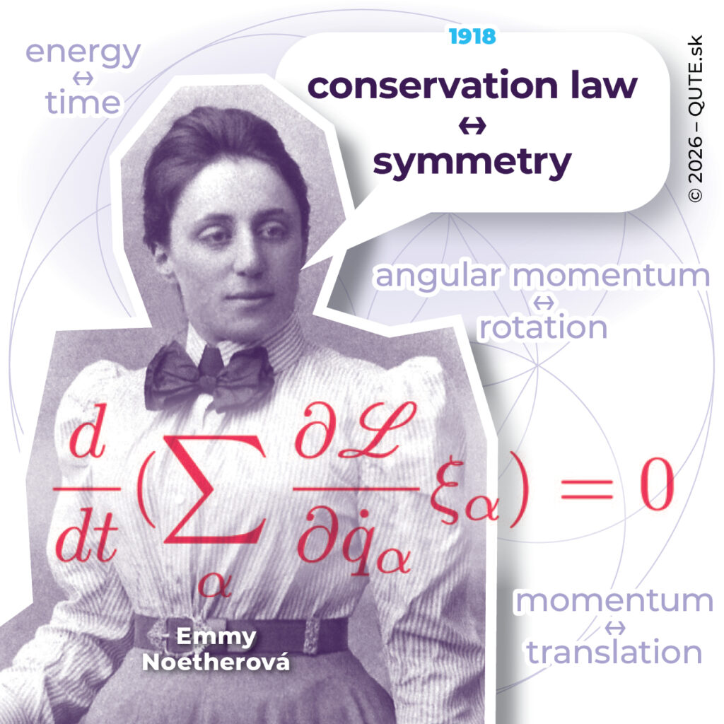
The connection between a system’s symmetry and conservation laws was discovered by mathematician Emmy Noether.
In 1918, German mathematician Emmy Noether showed that the conservation of energy is mathematically related to symmetry under time shifts – a second that passes today lasts just as long as a second that will pass tomorrow. In practice, this means that physical equations describing changes of system properties over time have this feature inherently built into them. This also applies to the equations of quantum physics.
Quantum formulas
However, there are some important specifics. How should we think about energy conservation when energy does not have definite values, and we can only talk about the probabilities with which different energy values may be observed? Moreover, these values are not arbitrary. “Formulas” do not always exist or behave in the way we are used to.
For example, the possible energy values of the hydrogen atom are given by Eg/n2, kde Eg= – 2.18×10⁻¹⁸ J is the ground-state energy and n=1,2,3,…n=1,2,3,…. No other values can be measured. The uncertainty relation between the energy of the hydrogen atom and the position or velocity of the electron implies that we cannot write a formula for energy in which velocity and position explicitly appear.
The situation is somewhat different for angular momentum, which is not in an uncertainty relation with the energy of the hydrogen atom. However, this is still not enough for a formula directly relating their values to exist. The magnitude of the total angular momentum of any system can take only the values L=√l(l+1)h/(2π) pre l=0,1/2,1,3/2,2, … . Quantum physics of the hydrogen atom requires that l≤n+1/2. For each energy, there are therefore several possible values of angular momentum, and the classical relation E=L2/(2mr2) – K/r for an electron orbiting a proton at a distance r, where K=2.31×10⁻²⁸ J.m, does not hold.
Time for amplitudes
Relationships between physical quantities in quantum physics do not take the form of simple formulas. This is because numbers themselves are not a fully suitable language for describing quantum properties. Even the fundamental equation of the quantum world – the Schrödinger equation – does not describe the time evolution of the values of physical quantities, nor their probabilities (those come from quantum predictions), but rather the evolution of their probability amplitudes.
Quantum uncertainty does not apply to the amplitudes of probabilities of different quantities. The probability amplitudes for energy values and those for position values are in a precise and well-defined mathematical relationship. We can say they are connected by formulas involving numbers, but these numbers do not describe the values of energy or position themselves – they describe only the amplitudes of their probabilities. If we know the probability amplitudes for one quantity, we can use these relations to compute the amplitudes for any other quantity.
These amplitudes define the quantum state of a system – everything we can know about the system in quantum physics. We denote the state by the symbol |ψ⟩. Knowing the state allows us to predict the probabilities of the outcomes of any measurement. If we want to predict how the state evolves in time, we must, in addition to knowing the state, solve the Schrödinger equation. What does that mean?
Hamiltonian
This equation, in the form of the so-called Hamiltonian, contains information about the “energetics” of the entire system. The Hamiltonian is not a quantum invention – the same concept appears in the same role in Newtonian, Maxwellian, and Einsteinian equations, among others. It is also called the generator of time evolution, because the equations in a sense express an equality between it and the time change of the system’s properties.
In the quantum case, it is the amplitudes and probabilities of physical quantities that change over time. These changes are fully deterministic and contain no element of randomness. Conservation of energy does not mean that amplitudes remain constant, but that the probabilities of the individual energy values of the system are preserved.
The actual energy values that we observe in measurements do not change and are encoded in the Hamiltonian together with the so-called energy basis of the system – states in which the system has a precisely defined energy value. In such states, the amplitudes of all possible energies except one are zero. Measuring a system in such an “energy” state therefore yields only a single possible outcome.
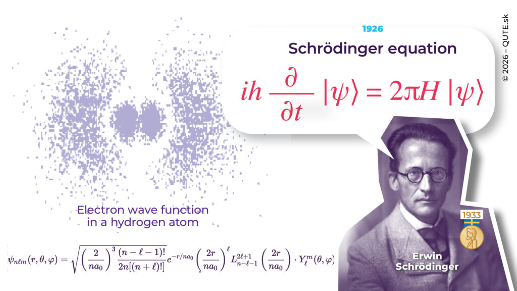
The main goal of research in the physics of the microscopic world is to decode the Hamiltonian – that is, to find its energy values and the corresponding energy states. In 1926, Erwin Schrödinger was the first to uncover the fundamental equation of the quantum world. After formulating the equation for the hydrogen atom, he solved this problem by identifying its possible energy values, which matched experimentally known results.
Schrödinger equation – its solutions take the form of wave functions. The example shown represents the energy states of the hydrogen atom and an illustration of the electron’s probability distribution in one of these states.
Modeling the quantum world
The number of systems for which we can truly solve the Schrödinger equation can be counted on the fingers of one hand. In most cases, our solutions rely on approximate computational methods and the power of computers. In the 1980s, Richard Feynman realized that existing computers would not be effective in modeling quantum systems and proposed the idea of using quantum systems themselves for simulation.
Simulations of quantum systems are not merely an academic pastime. By solving the Schrödinger equation, we understand the properties of materials, discover new technologies, and speak of chemistry as applied physics. A quantum computer is not only a threat to cryptographic systems; its primary utility is expected to lie precisely in the simulation of natural processes, which are quantum by their very nature.
Author of the article: Mário Ziman, Institute of Physics, Slovak Academy of Sciences, Bratislava
Illustrations: Diana Cencer Garafová, QUTE.sk – Slovak National Center for Quantum Technologies
Image source: wikipedia public domain

